- 8777701917
- info@saikatinfotech.com
- Basirhat W.B

In a Fiber-to-the-Home (FTTH) network, optical power levels are crucial for ensuring efficient transmission of data between the Optical Line Terminal (OLT) at the service provider’s central office and the Optical Network Terminal (ONT) at the customer’s premises. These power levels are typically measured in dBm (decibels relative to milliwatts), and they must fall within certain ranges to maintain reliable communication and avoid signal degradation.
Here’s a detailed list of typical optical power levels (in dBm) for FTTH systems:
The OLT is located at the service provider’s central office and transmits data to multiple ONTs over a Passive Optical Network (PON). The power output from the OLT is designed to reach all the ONTs within the PON coverage area, taking into account fiber attenuation, splitters, and other losses.
These values represent the optical power sent from the OLT to all ONTs in the network. The OLT transmits over a fiber network, and the optical power must be sufficient to overcome fiber loss and reach the customer premises.
The ONT (or ONU, Optical Network Unit) is located at the customer’s premises and receives the optical signal from the OLT via the PON. The ONT is responsible for converting the optical signal into electrical signals for use by end-user devices such as computers, phones, and TVs.
These power levels are the receive power that the ONT is designed to handle. Too high a power level can damage the ONT, while too low a power level may lead to poor signal quality or complete signal loss.
The ONT transmits data back to the OLT in the upstream direction. The power output of the ONT in the upstream direction is much lower than the downstream power output because the OLT is more sensitive and can receive lower power levels.
These values represent the optical power the ONT transmits back to the OLT. The OLT receives this weaker signal and processes it accordingly.
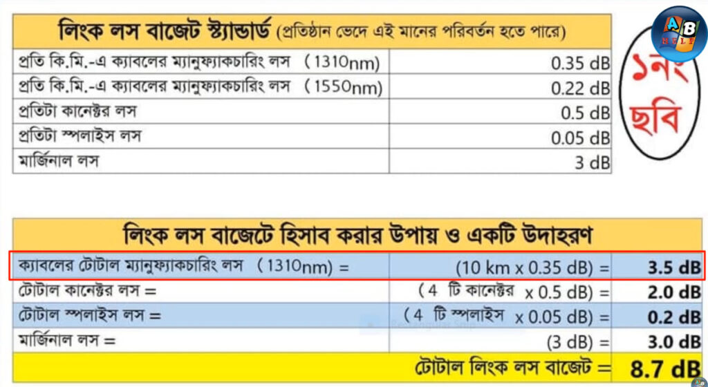
The link budget refers to the total loss (in dB) between the OLT and ONT. It takes into account factors like fiber attenuation, splitter losses, and connector losses. A typical FTTH link budget ensures that the signal remains strong enough to maintain a reliable connection.
The OLT must output enough power to compensate for all these losses and still ensure that the ONT receives a signal within the acceptable range.
Here are the minimum and maximum allowable optical power levels for the components in FTTH systems to ensure proper operation:
| Component | Direction | Typical Power Range (dBm) | Description |
|---|---|---|---|
| OLT (PON Port) | Downstream | +3 dBm to +5 dBm | Power output from OLT to ONTs (downstream). |
| OLT (PON Port) | Downstream | +7 dBm (maximum) | Max output, higher values may damage ONT. |
| ONT/ONU | Downstream | -27 dBm to -23 dBm | Power reception at ONT from OLT (downstream). |
| ONT/ONU | Downstream | -20 dBm (maximum) | Max input, higher values may damage ONT. |
| ONT/ONU | Upstream | +1 dBm to +5 dBm | Power output from ONT to OLT (upstream). |
| ONT/ONU | Upstream | +6 dBm (maximum) | Max output, higher values may cause interference or damage to OLT. |
The fiber link loss is a key factor in the power budget. It depends on:
Typical fiber losses are:
A typical GPON system can support distances of up to 20 km with fiber loss compensation included in the link budget, while XG-PON and NG-PON2 are designed for both short and long distances, with the link budget optimized for higher speeds.
Here’s a quick summary of typical optical power levels for FTTH systems:
| Component | Direction | Typical Power Range (dBm) |
|---|---|---|
| OLT (Downstream) | Downstream | +3 dBm to +5 dBm |
| ONT (Downstream) | Receive (Downstream) | -27 dBm to -23 dBm |
| ONT (Upstream) | Upstream | +1 dBm to +5 dBm |
| OLT (Maximum Output) | Downstream | +7 dBm (maximum) |
| ONT (Maximum Input) | Receive (Downstream) | -20 dBm (maximum) |
Maintaining the correct power levels ensures that the OLT can communicate effectively with multiple ONTs over long distances without signal degradation or hardware damage. Proper power management, along with consideration of the fiber link budget, is crucial for a reliable FTTH network.
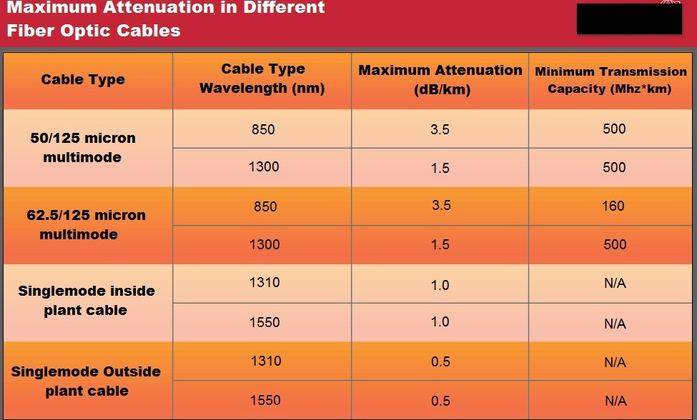
The fiber loss chart (or attenuation chart) shows the amount of signal loss that occurs over a fiber optic link due to various factors such as the type of fiber, wavelength, and distance. This loss is usually expressed in dB/km (decibels per kilometer) and can vary based on the type of fiber (single-mode or multi-mode) and the wavelength of light used for transmission.
The chart below provides typical attenuation values for single-mode fiber (SMF) and multi-mode fiber (MMF) at common wavelengths.
| Fiber Type | Wavelength (nm) | Attenuation (dB/km) |
|---|---|---|
| Single-Mode Fiber (SMF) | 850 nm | 3.0 to 3.5 dB/km |
| Single-Mode Fiber (SMF) | 1310 nm | 0.4 to 0.5 dB/km |
| Single-Mode Fiber (SMF) | 1550 nm | 0.2 to 0.3 dB/km |
| Multi-Mode Fiber (MMF) | 850 nm | 1.5 to 3.0 dB/km |
| Multi-Mode Fiber (MMF) | 1310 nm | 0.8 to 1.0 dB/km |
Single-Mode Fiber (SMF):
Multi-Mode Fiber (MMF):
The attenuation over a specific distance can be calculated using the following formula:
Loss (dB)=Attenuation (dB/km)×Distance (km)\text{Loss (dB)} = \text{Attenuation (dB/km)} \times \text{Distance (km)}Loss (dB)=Attenuation (dB/km)×Distance (km)
Single-Mode Fiber at 1550 nm:
Multi-Mode Fiber at 850 nm:
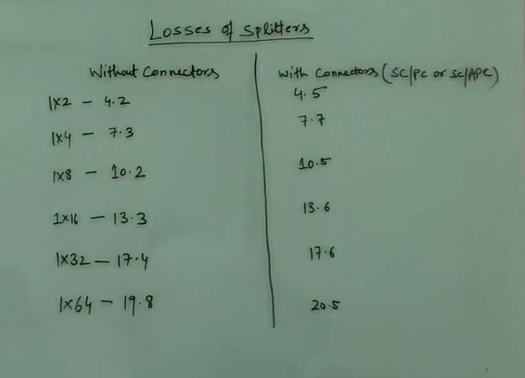
In addition to the inherent attenuation of the fiber itself, losses can also occur at fiber connectors, splices, and couplers. These are typically measured in dB and can add to the overall loss in the network.
Excessive bending of optical fibers can cause signal loss, referred to as bend loss. Tight bends in the fiber increase the attenuation, which can lead to significant signal degradation if not managed properly.
Here’s a graphical representation of the typical attenuation spectrum for single-mode fiber and multi-mode fiber:
| Fiber Type | Wavelength (nm) | Attenuation (dB/km) | Typical Usage |
|---|---|---|---|
| Single-Mode Fiber (SMF) | 850 nm | 3.0 to 3.5 dB/km | Short-range applications (LAN, internal networks) |
| Single-Mode Fiber (SMF) | 1310 nm | 0.4 to 0.5 dB/km | Medium-range applications (telecom, local internet) |
| Single-Mode Fiber (SMF) | 1550 nm | 0.2 to 0.3 dB/km | Long-range applications (backbones, FTTH, long-distance communication) |
| Multi-Mode Fiber (MMF) | 850 nm | 1.5 to 3.0 dB/km | Short-range applications (data centers, LAN) |
| Multi-Mode Fiber (MMF) | 1310 nm | 0.8 to 1.0 dB/km | Medium-range applications (campus networks) |
The fiber loss chart helps to understand the attenuation characteristics of fiber optics and is essential for designing efficient optical communication systems. When planning a fiber-optic link, consider both the fiber type and wavelength to select the best combination for your distance, performance, and cost requirements. For long-distance communication, single-mode fiber at 1550 nm is optimal due to its low attenuation, while for shorter distances, multi-mode fiber can be a more cost-effective solution despite higher attenuation.

Fiber optics has been providing long distance connections for a long time. But, until now, the higher cost often made it impractical in many LAN topologies. That is has been changing as the need for bandwidth rises and the price of fiber drops. Fiber is now moving into applications that were formerly the preserve of copper cable and it brings a number of significant advantages with it:
And, working with fiber keeps getting easier. New termination techniques, new splicing techniques, and new Small Form Factor (SFP) connector/termination products are making life a lot simpler for fiber installers. It is expected that costs for integrating fiber will be at par with Category 5 within a few years. Considering fiber’s many advantages, it is time to start planning ahead.
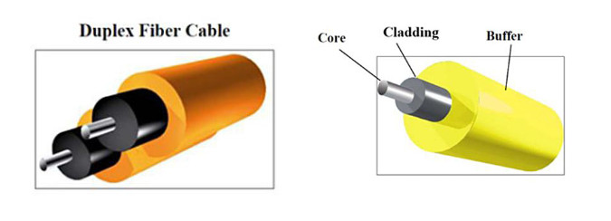
Fiber optic cable consists of three components:
The light signal is injected into the fiber via an LED, VCSEL or laser. For installations demanding higher power/quality, the transmitter will usually use a laser.
Multi-mode fiber is the most common fiber type used for network backbone inside buildings. It is the fiber type that the IEEE, ANSI, TIA, and ISO standards typically define in fiber LAN specifications.
The most commonly installed multi-mode core size is 62.5 micrometers (μm). The associated cladding size is 125 μm. But other core sizes are available, like 50 μm, 100 μm, 62.5/125 μm, and 50/125 μm.
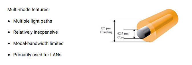
The ‘multi’ in multi-mode comes from the fact that light travels down the cable in multiple paths. The light beam “bounces” off the cladding as it travels down the core. That means that signals do not necessarily arrive at the receiver at the same instant. Called “modal dispersion”, it is the reason multi-mode fiber has less range than single-mode.
There are two distinct multi-mode methods:
Graded index is the current standard used by nearly all LAN/WAN equipment. Because of the light transmission characteristics of multi-mode, the quality of the fiber cable need not be high. In addition, multi-mode transmitters are relatively inexpensive.
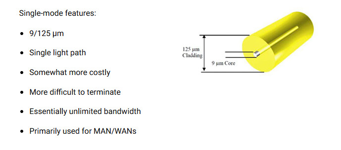
Single-mode fiber is used in more demanding applications. Single-mode uses a smaller core diameter (between 8 and 12 μm, with 9 μm being the average) and the same cladding diameter as multi-mode fiber.
Fiber optic cables use several different wavelengths to carry Ethernet:
The following table shows the different fiber optic standards as defined by the IEEE.
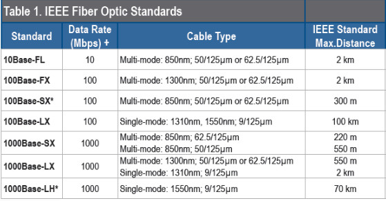
+ 4B5 encoding on Fast Ethernet and Gigabit Ethernet result in actual bit rates of 125 Mbps and 1250 Mbps respectively.
*100Base-SX (short wavelength multi-mode) and 1000Base-LH (long-haul single-mode) are not formally adopted standards, but are commonly understood and used in fiber optic networking.
To keep it simple, let’s discuss data transmitted over a fiber link is if it were always Full-Duplex (FDX). In a Half-Duplex (HDX) environment, the timing considerations limit the fiber link distances and these limitations apply no matter what fiber is being used.
Since there are two distinct types of fiber cable and three commonly used wavelengths (850 nm, 1300 nm, 1550 nm), the attenuation measurement will vary according to the cable and wavelength being used. Attenuation is measured in dB and is either quoted as attenuation in dB/km, or via an attenuation chart giving the attenuation for the entire fiber run. Note that the decibel scale is logarithmic – a loss of 99% of the light over a given length of fiber is expressed as “-20 dB”, a loss of 99.9% is “-30 dB”, and so forth.
• Attenuation – Fiber cabling has losses from absorption and back reflection of the light caused by impurities in the glass. Attenuation is a function of wavelength and needs to be specified for the particular wavelength in use.
• Modal Dispersion – The higher the data rate, the shorter the distance that the signal can travel before modal dispersion makes it impossible to distinguish between a “1” and “0”. Modal dispersion is only a concern with multi-mode cable and is directly proportional to the data rate.
• Dispersive Losses – While single-mode fiber is not subject to modal dispersion, other dispersion effects cause pulse spreading and limit distance as a function of data rate. Chief among these is “chromatic dispersion,” where the broader spectrum of certain transmitter types can result in varying travel times for different parts of a light pulse. Chromatic dispersion typically only starts to become a limiting factor at Gigabit speeds.
• Splices – Although losses can be small, and often insignificant, there is no perfect lossless splice. Many errors in loss calculations are the result of a failure to include splices. Average splice loss in single-mode cable is usually less than 0.01 dB.
• Connectors – Like splices, there is no perfect lossless connector. It is important to note that even the highest quality connectors can get dirty. Dirt and dust can completely obscure a fiber light wave and create huge losses. Typically, connector loss can vary from 0.15 dB (LC) to 0.5 dB (ST-II). Calculating for a 0.5 dB loss per connector is common and typically represents the worst case scenario, assuming that a cleaned and polished connector is used. Note that there will always be a minimum of two connectors per fiber segment, so remember to multiply connector loss by two.
• Safety Buffer – Add a couple dB of loss as a design margin. Allowing for 2 or 3 dB can account for fiber aging, poor splices, temperature and humidity.
Failure to account for one of these variables can create potential problems. Always test and validate the losses once the fiber is laid. Note that all calculations assume Full-Duplex (FDX) mode of operation.
The numbers listed below are averages and standard for new fiber. Actual numbers may vary for any installation.
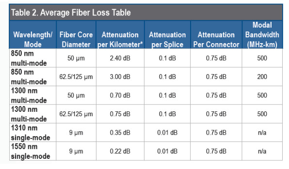
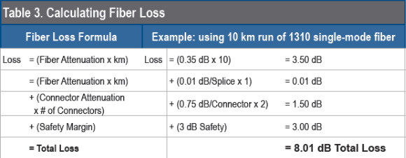
There are two different calculations required with fiber. Each assumes that there are known values for different sets of variables.
Calculate maximum signal by loss finding the sum of all worst case variables within a fiber segment. The numbers shown in the table above are average losses. Actual losses could be higher or lower depending upon many factors.
Calculating the signal strength exiting a cable is only half the job. To avoid overdriving a fiber receiver and to eliminate data loss, you must also calculate the “maximum signal strength.” Overdriving a receiver is most common when using single-mode products with very low fiber attenuation. It is safe to assume average numbers for fiber loss but, to verify previous measurements and avoid performance problems, the actual losses should be measured once the fiber has been deployed,
Calculating fiber distance involves the loss variables described above as well as the launch power and receive sensitivity specifications on the fiber products. When calculating distance, use the lowest launch power on the vendor’s specifications to calculate a worst case distance. Use the highest specified launch power to ensure the receiver is not being overdriven.
Start by calculating the power budget. This is found by subtracting the receive sensitivity from the launch power.
Power Budget = (Launch Power) – (Receive Sensitivity)
For example, assume a fiber switch with a –17 dBm minimum launch power is connecting to a media converter with a worst case receive sensitivity of 30 dBm:
Power Budget = (-17 dBm) – (-30 dBm) = 13 dB
It may seem odd that subtracting two numbers with dBm as the unit of measure results in a number with dB as the unit of measure. This is because a dBm is a logarithmic ratio of power relative to 1 mW. Subtraction of two logarithmic ratios is the equivalent of dividing the two power measurements directly, resulting in a unitless number expressed in dB.
Because power budgets can be calculated using either decibels or Watts, it is useful to know how to convert between decibels (dBm) and Milliwatts (mW). The two formulas are shown below:
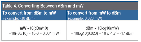
The power budget formula can be expressed in mW rather than dBm. Using the dBm to mW conversion shown above, -17 dBm becomes 0.020mW, -30 dBm becomes 0.001mW and, since subtracting logarithms is the equivalent of dividing two regular numbers, the formula becomes:
Power Budget = 0.020 mW/0.001 mW = 20
This means the system can sustain a total loss of 95% of the transmitted light or that 1/20th of the transmitted light must reach the receiver. The use of dB and dBm as units allows addition and subtraction of reasonably sized numbers rather than multiplication and division of very large or very small numbers.
For a given power budget for 850nm 50 μm multi-mode fiber, and making some assumptions about the number of splices and connections, it is possible to estimate the distance that a fiber with particular specifications can run. For example, using the numbers from above:
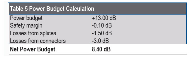
If the fiber is specified at a loss not to exceed 2.5 dB/km:
(8.40 dB) / (2.5 dB/km) = 3.36 km
The fiber can be run for approximately 3.36 km (2.1 mi) before running out of signal strength at the end.
Multi-mode cable tends to disperse a light wave unevenly and can create a form of jitter as the data traverses the cable. This jitter tends to create data errors as the data rate increases.
In addition to calculating budget across multi-mode fiber, it is also necessary to calculate the losses resulting from modal dispersion. The maximum length of fiber will be determined by distance calculation (above) or by modal dispersion – whichever is lowest.
For example, assume the network is using 100 Mbps Fast Ethernet (which has an actual bit rate of 125 Mbps) across 850 nm multi-mode fiber. The modal dispersion of this multimode cable is 200 MHz-km. Use the following equation to calculate the maximum distance of a 125 Mbps (MHz) Fast Ethernet signal:
Distance = 200 MHz-km/125 MHz = < 1.6 km
Similarly, calculating the maximum distance at a 10 Mbps Ethernet data rate:
Distance = 200 MHz-km/10 MHz = < 20.0 km