Overview Fiber Optic

Fiber optic cables are used for high-speed data transmission over long distances. They rely on light signals (usually infrared) to transmit data, and they can be made from glass or plastic fibers. The two main categories of fiber optic cables are single-mode and multi-mode, and each type has its own advantages, uses, and characteristics.

Here’s a detailed breakdown of fiber optic cable types, including their construction, performance, and use cases:

1. Single-Mode Fiber (SMF)

  • Core Diameter: 8-10 microns
  • Cladding Diameter: 125 microns (standard for all fiber cables)
  • Light Transmission: Uses laser light sources (typically 1310 nm or 1550 nm wavelengths).
  • Transmission Range: Designed for long-distance transmission (up to 40 km or more, depending on the equipment and wavelength).
  • Bandwidth: Higher bandwidth than multi-mode fiber, supporting faster data rates over longer distances.
  • Cost: Generally more expensive than multi-mode fiber due to precision manufacturing and components.
  • Performance: Single-mode fiber experiences less signal loss and dispersion compared to multi-mode fiber, making it ideal for long-distance, high-speed networks.

Common Uses:

  • Telecom networks
  • Long-haul connections (inter-city, between data centers)
  • Internet backbone networks
  • High-speed Ethernet (10 GbE, 40 GbE, 100 GbE)
  • Fiber to the home (FTTH) or fiber to the building (FTTB)

2. Multi-Mode Fiber (MMF)

  • Core Diameter: Typically 50 or 62.5 microns (much larger than single-mode fiber).
  • Cladding Diameter: 125 microns.
  • Light Transmission: Uses LED light sources (usually 850 nm or 1310 nm wavelengths).
  • Transmission Range: Optimized for shorter distances (up to 2 km for 10G Ethernet; less for higher-speed protocols like 40GbE or 100GbE).
  • Bandwidth: Generally lower bandwidth than single-mode fiber, especially over long distances, due to signal dispersion (modal dispersion).
  • Cost: Multi-mode fiber is less expensive than single-mode fiber, both for the cable itself and the equipment (such as transmitters and receivers).

Common Uses:

  • Data centers (for intra-rack, inter-rack, and short-distance links)
  • Local area networks (LANs)
  • Enterprise networks
  • High-speed Ethernet (1 GbE, 10 GbE, 40 GbE, 100 GbE) over shorter distances
  • Building-to-building connections within a campus network

Key Differences Between Single-Mode and Multi-Mode Fiber:

PropertySingle-Mode Fiber (SMF)Multi-Mode Fiber (MMF)
Core Size8-10 microns50 or 62.5 microns
Light SourceLaser (more focused beam)LED (less focused beam)
WavelengthTypically 1310 nm or 1550 nmTypically 850 nm or 1310 nm
Transmission DistanceLong-distance (up to 40+ km)Short-distance (up to 2 km)
BandwidthHigher bandwidth, less signal degradationLower bandwidth, higher modal dispersion
CostMore expensive (both cables and equipment)More affordable (cables and equipment)
ApplicationsLong-distance, high-speed applications (e.g., internet backbone, telecom)Short-distance applications (e.g., data centers, LANs)

3. Fiber Optic Cable Types Based on Construction:

a. Simplex Fiber Optic Cable

  • Configuration: Contains a single fiber (one core and one cladding).
  • Direction of Transmission: Unidirectional — used for one-way communication (data can only travel in one direction at a time).
  • Use Cases:
    • Telecommunications: Point-to-point connections.
    • Sensor networks: Simple, low-cost applications requiring one-way data transmission.

b. Duplex Fiber Optic Cable

  • Configuration: Contains two fibers (one for transmitting and one for receiving signals).
  • Direction of Transmission: Bidirectional — can carry data in both directions simultaneously.
  • Use Cases:
    • Ethernet connections.
    • Fiber optic networking for data centers or backbone links where bidirectional communication is needed.

c. Multicore Fiber Optic Cable

  • Configuration: Contains multiple cores within a single cable, allowing for multiple independent channels within one fiber cable.
  • Use Cases:
    • High-density installations.
    • Telecom networks that need to increase the number of fiber paths in a limited space.
    • High-capacity networking (multiple wavelengths or data streams).

d. Ribbon Fiber Optic Cable

  • Configuration: Contains multiple fibers (arranged in flat, ribbon-like structures), where each ribbon can have multiple individual fibers, typically 12 or 24 fibers per ribbon.
  • Use Cases:
    • High-density fiber installations.
    • Data centers or high-volume networking environments where a large number of fibers need to be routed in a compact form.

e. Armored Fiber Optic Cable

  • Configuration: Designed with protective armor (usually a metal layer) around the fiber to protect it from physical damage, making it suitable for outdoor or harsh environments.
  • Use Cases:
    • Outdoor installations.
    • Industrial environments where physical damage (e.g., from rodents or machinery) is a risk.
    • Underground deployments where protection from impact and pressure is needed.

4. Other Key Fiber Optic Cable Characteristics:

a. Fiber Optic Cable Jacket Types:

  • LSZH (Low Smoke Zero Halogen): Safe for indoor environments, produces minimal smoke in the event of a fire.
  • PVC (Polyvinyl Chloride): Standard jacket material, suitable for dry indoor environments.
  • PE (Polyethylene): Used for outdoor and direct burial cables, often with an added layer of water-blocking material.

b. Fiber Optic Cable Coating:

  • Primary Coating: Surrounds the core and cladding, typically made of soft acrylate material to protect the fibers from damage.
  • Secondary Coating: Provides extra protection and may be a tougher material.
  • Strength Members: Provides strength to the cable, often made from Kevlar or steel.

5. Fiber Optic Cable Applications:

  • Telecommunications Networks: Fiber optic cables are essential for long-distance voice, video, and data transmission in modern telecom systems.
  • Internet Backbone: They provide the high-speed data transfer backbone for large internet service providers (ISPs) and data centers.
  • Data Centers: MMF cables are commonly used for short-range, high-speed connections between switches, routers, and servers in data centers.
  • FTTH (Fiber to the Home): Fiber optics is increasingly being used to deliver high-speed internet directly to homes and businesses.
  • Military and Aerospace: Fiber optics are used for secure and high-bandwidth communication in sensitive or rugged environments.
  • Industrial and Medical: Special types of fiber optics are used for high-precision measurement, sensing, and monitoring applications.

Conclusion:

Fiber optic cables are an essential part of modern communication networks, offering high-speed, high-capacity, and long-distance data transmission. Understanding the types of fiber (single-mode vs. multi-mode), their construction, and their use cases will help you choose the right fiber optic cable for your network needs, whether it’s for a telecom network, data center, local area network (LAN), or industrial application.

Fiber Patch Coard


A fiber optic patch cord (also known as a fiber optic jumper or fiber patch cable) is a short cable used to connect devices such as switches, routers, fiber optic panels, or other optical network equipment. It consists of fiber optic cables with connectors at both ends. These patch cords are used in data centers, telecom networks, and other environments to enable flexible fiber optic connections.

Fiber optic patch cords are generally classified based on several factors, including the fiber type, connector type, and length. Below is an overview of the main types of fiber optic patch cords:

1. Fiber Type in Patch Cords:

Fiber optic patch cords can either be single-mode or multi-mode, and this depends on the type of fiber used inside the cable.

a. Single-Mode Fiber (SMF) Patch Cords:

  • Core Diameter: Typically 8-10 microns.
  • Wavelength: Typically designed for 1310 nm or 1550 nm transmission.
  • Applications: Used in long-distance communication, telecom networks, high-speed internet backbones, and long-haul data connections.
  • Performance: Lower loss, higher bandwidth, and better performance over long distances compared to multi-mode fiber.
  • Use Case: Ideal for telecom applications and long-range networking in data centers, telecom exchanges, and fiber optic backbone infrastructures.

b. Multi-Mode Fiber (MMF) Patch Cords:

  • Core Diameter: Typically 50 µm or 62.5 µm.
  • Wavelength: Typically operates at 850 nm or 1310 nm.
  • Applications: Used for short to medium-distance connections in data centers, LANs, and campus networks.
  • Performance: Higher signal dispersion than single-mode, making it suitable for shorter distances (up to a few hundred meters for higher-speed networks).
  • Use Case: Perfect for data center interconnects, short-distance Ethernet links, and local area networks (LANs).

2. Connector Type in Patch Cords:

The type of connector used on both ends of the fiber optic patch cord is crucial for determining the compatibility and application of the patch cord. Here are the most common fiber optic connectors used in patch cords:

a. SC (Subscriber Connector)

  • Design: Square, push-pull design, which is easy to use.
  • Applications: Common in telecom and datacom applications.
  • Features: Low-cost, high-performance, and widely used in fiber-to-the-home (FTTH) installations, network equipment, and in data centers.

b. LC (Lucent Connector)

  • Design: Smaller than SC connectors (1.25 mm ferrule) and typically used in high-density installations.
  • Applications: Data centers, network switches, and high-performance computing (HPC) environments.
  • Features: Smaller form factor, often used in duplex (two fibers in one cable) configurations.

c. ST (Straight Tip)

  • Design: Bayonet-style connector.
  • Applications: Used in older telecom systems and high-frequency applications.
  • Features: Relatively easy to install, but being replaced in modern networks by LC and SC connectors.

d. MTP/MPO (Multi-fiber Push On/Pull Off)

  • Design: High-density connectors for multi-fiber cables (typically 12 or 24 fibers in a single connector).
  • Applications: Common in high-density data centers and backbone networks.
  • Features: Allows multiple fibers to be connected in one action, saving space and time for large-scale networks.

e. FC (Ferrule Connector)

  • Design: Threaded connector with a metal ferrule, often used for precision applications.
  • Applications: Used in telecom and high-precision instrumentation.
  • Features: Provides a secure connection with high performance and low insertion loss.

f. E2000 Connector

  • Design: Push-pull locking mechanism similar to SC but with better performance.
  • Applications: High-end telecom networks and fiber optic communication systems.
  • Features: Provides high return loss, often used in environments where high performance is required.

3. Patch Cord Construction:

Fiber optic patch cords are typically made of a fiber optic cable with connectors at each end. They are available in simplex or duplex configurations:

a. Simplex Patch Cord:

  • Configuration: One fiber for one-way communication.
  • Use Case: Single-channel connections where data is transmitted in one direction at a time.
  • Common Applications: Point-to-point connections, single-channel communications.

b. Duplex Patch Cord:

  • Configuration: Two fibers, one for transmitting and one for receiving data, enabling bidirectional communication.
  • Use Case: Most common type of patch cord in networking, supporting bi-directional traffic.
  • Common Applications: Ethernet, Fibre Channel, telecom systems, and data center interconnections.

c. Simplex vs. Duplex:

  • Simplex is used for single-direction data transmission, while Duplex allows for two-way data transmission.
  • Duplex patch cords are used for most applications in modern networking.

4. Common Fiber Optic Patch Cord Specifications:

AttributeSingle-Mode Fiber Patch CordMulti-Mode Fiber Patch Cord
Core Diameter8-10 µm50 µm or 62.5 µm
Transmission Wavelength1310 nm, 1550 nm850 nm, 1310 nm
Transmission DistanceLong-distance (up to 40 km or more)Short to medium-distance (up to 2 km for 10GbE)
BandwidthHigher (less signal dispersion)Lower (higher dispersion at longer distances)
Connector TypeSC, LC, FC, MTP/MPOSC, LC, ST, MTP/MPO
Common UsesLong-haul networks, high-speed backbonesData centers, LANs, short-distance links

5. Length of Fiber Optic Patch Cords:

Fiber optic patch cords come in various lengths, and the length required depends on the specific installation. Typical lengths range from 1 meter to 10 meters, but they can be custom-made to fit particular needs.

6. Performance Factors:

Insertion Loss:

  • This refers to the signal loss that occurs when light is transmitted through the patch cord. Low insertion loss is crucial for high-performance networks.
  • Single-mode patch cords typically have lower insertion loss than multi-mode patch cords.

Return Loss:

  • Return loss measures the amount of light reflected back towards the source. A high return loss value indicates good performance, as less light is reflected.

Attenuation:

  • Attenuation is the reduction in signal strength over distance. Single-mode cables have lower attenuation compared to multi-mode cables.

Summary of Fiber Optic Patch Cord Types:

Fiber TypeConnector TypesApplications
Single-Mode Fiber (SMF)SC, LC, ST, FC, MTP/MPOLong-distance networking (telecom, internet backbone, etc.)
Multi-Mode Fiber (MMF)SC, LC, ST, MTP/MPOShort-distance networking (data centers, LANs, etc.)
SimplexSC, LC, ST, FCSingle-direction communications
DuplexSC, LC, ST, MTP/MPOBidirectional communications (common in modern networks)

Conclusion:

Fiber optic patch cords are essential components in modern networking, enabling quick and flexible connections between devices in data centers, telecom networks, and other high-speed communication systems. Choosing the right type of fiber optic patch cord—based on fiber type (single-mode or multi-mode), connector type, and length—ensures optimal performance and reliability for specific network applications.


Types of Multimode Fiber:

As standard ISO 1180 identifies, we can classify MMF optic cables into OM1 Optical Fiber, OM2 optical fiber, OM3 optical fiber, OM4 optical fiber and the modern OM5 optical fiber. The following part will analyze these fiber optics from the angle of bandwidth, core size, distance, data rate, optical source, and color in detail.

OM1 Optical Fiber:

OM1 optical Fiber has a 62.5 µm core size, and the color of its jacket is orange. It supports 10GbE at 33m lengths. We mainly use it for 100Mbps Ethernet implementations. This type typically utilizes a light source of LED.

OM2 Optical Fiber:

The color of the OM2 fiber jacket is also orange, and it possesses a 50 µm core size. It can support 10GbE at 82m lengths, but we commonly use it for 1GbE implementations. It utilizes a light source of LED.

OM3 Optical Fiber:

The color of the OM3 fiber jacket is aqua, and it possesses a 50 µm core size, but we have optimized the cable for laser-based equipment. This type of fiber supports 10GbE at 300m lengths. However, we commonly use 10GbE. Nevertheless, OM3 can help 40G and 10GbE to 100m.

OM4 Optical Fiber:

This fiber is backward adaptable to OM3 optical fiber and possesses a similar aqua jacket. We have developed OM4 specifically for laser transmission of VCSEL, enabling 10 Git/s connection ranges to 550 meters, contrary to 300 meters with OM3. Moreover, it can extend from 40/100GB to 150m using an MPO connector.

OM5 Optical Fiber:

We can also signify this type of fiber as wideband MMF (WB MMF). OM5 is the modern type of MMF and is backward adaptable to OM4. It possesses a similar core size to OM4, OM3, and OM2. OM5 fiber’s jacket color is lime green. We have designed and specified it to support four channels of WDM at 25Gbps speed per channel via 850-950 nanometers window.

Differences between OM1, OM2, OM3, OM4, and OM5:

The main difference between multimode optical fibers lies in physical contrasts. Therefore, physical difference causes different communication data rate and range. Watch this video to understand the distinctions between OM1 fiber, OM2 fiber, OM3 fiber, OM4 fiber, and OM5 fiber.

Physical Distinction:

The physical difference mainly rests upon jacket color, diameter, bandwidth, and optical source, which we have described in the table below.

There are different types of fiber optic cable. Some types are single-mode, and some types are multimode. Multimode fibers are described by their core and cladding diameters. Usually the diameter of the multimode fiber is either 50/125 µm or 62.5/125 µm. At present, there are four kinds of multi-mode fibers: OM1, OM2, OM3 and OM4. The letters “OM” stand for optical multimode. Each type of them has different characteristics.Multimode fibers are identified by the OM (“optical mode”) designation as outlined in the ISO/IEC 11801 standard.Their difference is following:


Standard:

Each “OM” has a minimum Modal Bandwidth (MBW) requirement. OM1, OM2, and OM3 fiber are determined by the ISO 11801 standard, which is based on the modal bandwidth of the multimode fiber. In August of 2009, TIA/EIA approved and released 492AAAD, which defines the performance criteria for OM4. While they developed the original “OM” designations, IEC has not yet released an approved equivalent standard that will eventually be documented as fiber type A1a.3 in IEC 60793-2-10.


Differences:

OM1, for fiber with 200/500 MHz*km overfilled launch (OFL) bandwidth at 850/1300nm (typically 62.5/125um fiber)

OM2, for fiber with 500/500 MHz*km OFL bandwidth at 850/1300nm (typically 50/125um fiber)

OM3, for laser-optimized 50um fiber having 2000 MHz*km effective modal bandwidth (EMB, also known as laser bandwidth), designed for 10 Gb/s transmission.

OM4, for laser-optimized 50um fiber having 4700 MHz*km EMB bandwidth designed for 10 Gb/s, 40 Gb/s, and 100 Gb/s transmission.


Diameter: The core diameter of OM1 is 62.5 µm , however, core diameter of the OM2, OM3 and OM4 is 50 µm.

Jacket Color: OM1 and OM2 MMF are generally defined by an orange jacket. OM3 and OM4 are usually defined with an aqua jacket.

Optical Source: OM1 and OM2 commonly use LED light source. However, OM3 and OM4 usually use 850 nm VCSELs.

Bandwidth: At 850 nm the minimal modal bandwidth of OM1 is 200MHz*km, of OM2 is 500MHz*km, of OM3 is 2000MHz*km, of OM4 is 4700MHz*km.


OM3 & OM4 are Superior to OM1&OM2

Both OM1 and OM2 work with LED based equipment that can send hundreds of modes of light down the cable, while OM3 and OM4 are optimized for laser (eg. VCSEL) based equipment that uses fewer modes of light. LEDs can not be turned on/off fast enough to support higher bandwidth applications, while VCSELs are capable of modulation over 10 Gbit/s and are used in many high speed networks. For this reason, OM3 and OM4 are the only multi-mode fibers included in the 40G and 100G Ethernet standard. Now OM1 and OM2 are usually used for 1G which are not suitable for today’s higher-speed networks. OM3 and OM4 are used for 10G mostly at present. But in the future, since OM3 and OM4 can support the 40G and 100G, which may make them the tendency.


Specifications:

OM1 cable typically comes with an orange jacket and has a core size of 62.5 micrometers (µm). It can support 10 Gigabit Ethernet at lengths up 33 meters. It is most commonly used for 100 Megabit Ethernet applications.

OM2 also has a suggested jacket color of orange. Its core size is 50µm instead of 62.5µm. It supports 10 Gigabit Ethernet at lengths up to 82 meters but is more commonly used for 1 Gigabit Ethernet applications.

OM3 fiber has a suggested jacket color of aqua. Like OM2, its core size is 50µm. It supports 10 Gigabit Ethernet at lengths up to 300 meters. Besides OM3 is able to support 40 Gigabit and 100 Gigabit Ethernet up to 100 meters. 10 Gigabit Ethernet is its most common use.

OM4 also has a suggested jacket color of aqua. It is a further improvement to OM3. It also uses a 50µm core but it supports 10 Gigabit Ethernet at lengths up 550 meters and it supports 100 Gigabit Ethernet at lengths up to 150 meters.

Fiber Wavelength Band

Optical fibers are the unsung heroes that make our broadband networks possible. These thin strands of ultra-pure glass carry unbelievable amounts of data across vast distances using beams of light.

The secret lies in the fiber’s ultra-low loss transmission windows at specific wavelength bands tailored to different network roles. Let’s shine a light on what makes each band unique.

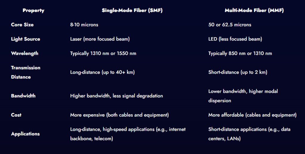
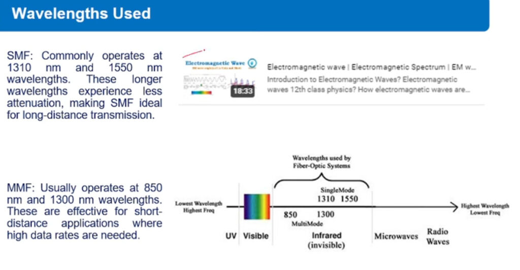
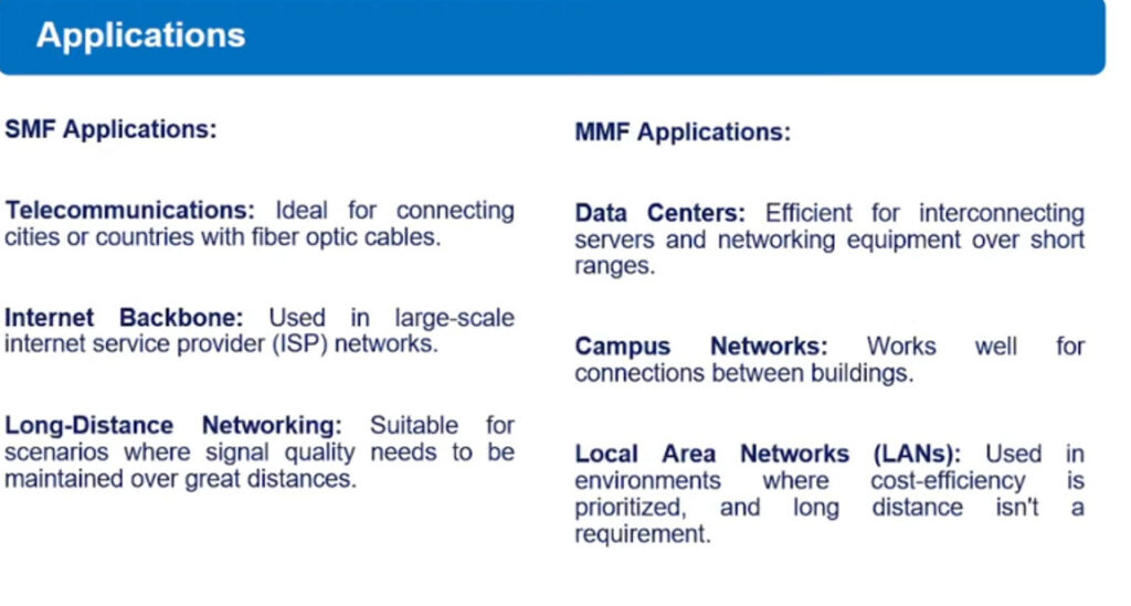
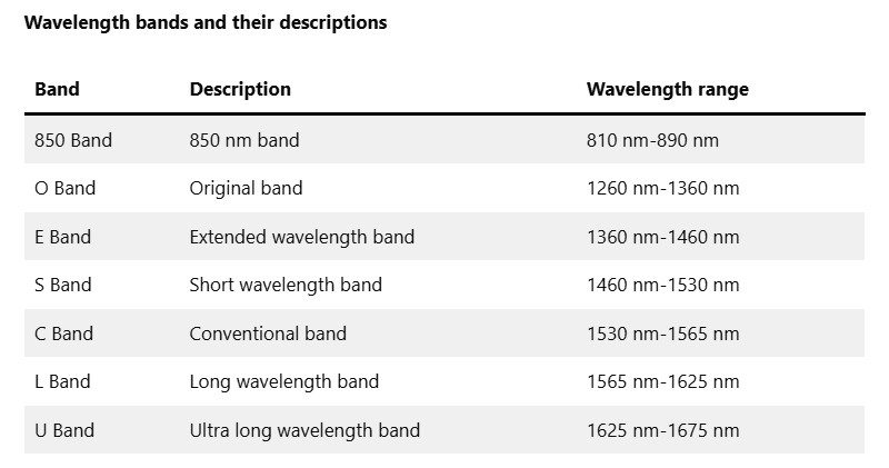
850 Band: The High-Speed Short Haul Workhorse

The 850 nanometer band covering 810-890 nm wavelengths was the first used for short, low-cost fiber links. It remains the prime choice for high bandwidth multidrop networks up to ~500 meters using cost-effective multimode fiber and Vertical-Cavity Surface-Emitting Laser (VCSEL) transmitters.

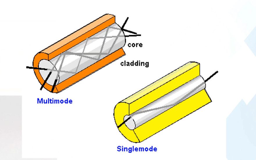
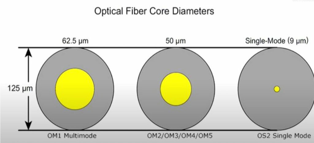
With a larger core than single-mode, multimode fiber allows multiple light ray paths for short reach. The 850 nm wavelength aligns perfectly with the peak efficiency curve of standard graded-index multimode fiber. This unlocks maximum bandwidth at minimum cost while simplifying the VCSEL transmitter.

The 850 nm band will continue serving as the high-speed workhorse inside data centers, corporate campuses, cell towers, aircraft infotainment, and automotive networking for decades to come.

O Band: Minimizing Loss and Distortion

The Original 1260-1360 nm band carries signals with minimum distortion across the greatest distances of any multimode band and sees loss on par with today’s single-mode fiber.

In a serendipitous quirk of physics, the O-band overlaps with an ultra-low-loss optical transmission window. It became the first wavelength for reliable long-haul telecom and cable TV in the late 1970s using early single-mode fiber.

The O-band also works well for shorter high-bandwidth runs up to ~1 km over multimode fiber. Its balance of low distortion and loss makes it a versatile choice for re-configurable enterprise and metro fiber networks

E Band: Pushing Fiber Performance

The extended 1360-1460 nm band emerged once fiber manufacturing achieved incredibly pure glass. Early fibers saw heavy E-band signal loss from residual water contamination.

Through a complex glass production refinement called vapor-phase dehydration, scientists reduced hydroxyl impurities. This opened the door to Zero Water Peak (ZWP) fibers optimized for the E band.

Today’s ultra-low-loss E Band matches or even exceeds the original O band performance. However, it took many years for equipment and networks to catch up following massive O band deployment.

Despite higher capacity potential, E band utilization still trails traditional bands, though it continues gaining ground in metro and regional optical networks.

S Band: Enabling Integrated Access Networks

The short wavelength 1460-1530 nm band strikes an optimum balance of low intrinsic fiber loss and component performance. It serves as the standard downstream data channel for many Passive Optical Network (PON) fiber access links.

PON technology powers Fiber-to-the-Home (FTTH) services by connecting many customers to a common fiber junction. The S-band downstream band ensures complete network isolation. Routing downstream 1490 nm S-band on one fiber and 1310 nm upstream/RF video on a second fiber prevents interference.

This enables economical triplexer modules serving all passive optical network signals from common fiber cable. It also allows upgrading deployed fiber without digging up existing routes or disrupting customers. The S-band continues bolstering broadband access capacity to meet demand.

C Band: The Global Telecom Workhorse

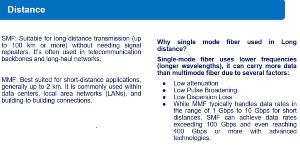
The conventional 1530-1565 nm band provides the lowest loss window across all single-mode telecom fibers, making it the dominant band for ultra-long-haul transport networks.

Modern 100G and 400G optical transmission leverages advanced modulation formats and spectrally efficient channel spacing. This requires the C band’s ultra-low attenuation to maintain adequate signal integrity across thousands of kilometers or more.

Global networks also rely on erbium-doped fiber amplifiers (EDFAs) and increasingly dense wavelength division multiplexing (DWDM) to boost capacity. Currently able to carry up to 72 x 400Gbps channels per fiber pair, the C band will continue to anchor tomorrow’s internet infrastructure, scaling to Zettabytes per second!

L Band: Doubling Network Capacity

The longer wavelength 1565-1625 nm band serves as vital spectrum headroom once C-band capacity maxes out between major hub sites.

Rather than laying more fiber, network operators add amplifiers, multiplexers, transceivers, and other optics optimized for the L-band as traffic growth dictates. This allows doubling capacity over existing routes by transmitting an additional 40+ super-channels alongside fully loaded C band systems.

Much of the existing fiber plant and EDFA amplifiers are L-band ready from inception. Turning up additional channels requires simple plugging in L-band components, making capacity easy to scale on-demand with minimal disruption.

U Band: Keeping Networks Healthy

The ultra-long wavelength 1625-1675 nm band lives in obscurity compared to mainstream telecom bands. It suffers from significantly higher intrinsic fiber attenuation, limiting its useful range.

However, the U band has emerged as the perfect stealth monitoring channel. All active links deploy inexpensive U-band diagnostics for round-the-clock health checks without disrupting revenue traffic.

Embedded U-band sensors analyze fiber loss, amplification gain, signal noise, chromatic and polarization mode dispersion, crosstalk, latency, and more. Network managers remotely log data and alerts to enhance quality, quickly catch degradation, and prevent outages.

So, while invisible to end users, the U band plays a vital role in ensuring robust networks. The same dark fiber and DWDM gear readily supports U-band monitoring alongside active telecom channels.

Wavelength Windows: Engineering Low Loss

Fiber optic networks balance distance with bandwidth, limited by attenuation and dispersion as photons propagate through glass. Telecom engineers optimize data rate and range by matching transmission bands to low-loss optical windows.

Windows are wavelength regions of ultra-low attenuation centered on bands from 850nm to 1675nm. Early systems exploited windows at:

  • 850nm for cheaper multimode fiber
  • 1300nm with minimum chromatic dispersion
  • 1550nm for single-mode long haul when attenuation rules

Fiber manufacturers relentlessly refined manufacturing, chasing purity to extend low-loss regions across the full spectrum. Chemical vapor deposition, precision preform drawing, hermetic jacketing, and innovations like vapor-phase dehydration tamed attenuation.

Today’s fibers achieve under 0.17 dB per km across the entire range up to 1675nm! This allows unregenerated transmission exceeding 300 km at 100Gbps across multiple bands.

Yet vestiges of historic windows persist in network architectures. Short reach favors 850nm for cost savings. Metro and regional networks balance the fiber generation mix by using multiple bands. Critical core links still run predominantly on the original 1550nm C-band for reliability – but not due to today’s fiber loss.

Rather than attenuation, amplification and multiplexing economics now anchor the C-band. Erbium-doped fiber amplifiers, Raman pumping, and dense WDM transport maximize capacity-distance products here. Other wavelengths achieve similar fiber loss yet lack ubiquitous optical gear support.

So next time you surf the net, take a moment to appreciate the ever-expanding low-loss windows that make our connected world possible!

Fiber Cable Core

Fiber optic cables are available with varying core (or fiber) counts to accommodate different network needs, from small-scale installations to large, high-capacity network infrastructure. The number of cores (fibers) in a cable determines its capacity for transmitting data and the number of independent channels it can support. The core count typically ranges from a few fibers to hundreds of fibers.

Common Fiber Core Counts and Their Applications:

1. Single-Core Fiber Optic Cable

  • Description: A cable with 1 fiber core.
  • Use Case: Rarely used in network installations because single fibers are often used as part of multi-fiber cables.
  • Applications: Point-to-point connections, custom installations, or test cables.

2. 2-Core Fiber Optic Cable

  • Description: Contains 2 fiber cores.
  • Use Case: Duplex cables, one core for transmit and the other for receive, used for bi-directional communication.
  • Applications: Simplex communication or fiber to the home (FTTH), short-range LAN connections, and telecommunications.

3. 4-Core Fiber Optic Cable

  • Description: Contains 4 fiber cores.
  • Use Case: Often used for local area networks (LANs), fiber optic patch cords, and short-range communication.
  • Applications: Used for fiber-to-the-building (FTTB) and small-scale network installations.

4. 6-Core Fiber Optic Cable

  • Description: Contains 6 fiber cores.
  • Use Case: Common for medium-density applications.
  • Applications: Used in data centers for small interconnections and medium-length building-to-building fiber links.

5. 12-Core Fiber Optic Cable

  • Description: Contains 12 fiber cores.
  • Use Case: Used in medium-density networks or short to medium distance applications.
  • Applications: Common in data centers, campus networks, and telecom backbones. Also used in fiber patch panels.

6. 24-Core Fiber Optic Cable

  • Description: Contains 24 fiber cores.
  • Use Case: For higher-density installations and larger networks.
  • Applications: Typically used in data centers, fiber backbone networks, and large campus networks.

7. 48-Core Fiber Optic Cable

  • Description: Contains 48 fiber cores.
  • Use Case: Used for high-capacity installations, capable of supporting multiple data channels in dense environments.
  • Applications: Common in telecom networks, large-scale data centers, and long-haul networking.

8. 72-Core Fiber Optic Cable

  • Description: Contains 72 fiber cores.
  • Use Case: Used for very high-capacity installations, often in high-performance data centers and backbone networks.
  • Applications: Large-scale fiber optic infrastructures, where a significant number of individual connections are needed.

9. 96-Core Fiber Optic Cable

  • Description: Contains 96 fiber cores.
  • Use Case: Ideal for large-scale network applications requiring massive data throughput.
  • Applications: Typically used in core networks, data center backbones, and telecom infrastructure.

10. 144-Core Fiber Optic Cable

  • Description: Contains 144 fiber cores.
  • Use Case: Used in high-density network environments that need to accommodate a huge number of connections in a compact form factor.
  • Applications: Often seen in large data centers, central offices, and telecom operator infrastructure.

11. 288-Core Fiber Optic Cable

  • Description: Contains 288 fiber cores.
  • Use Case: Extremely high-density installations, often for core networking or fiber optic distribution systems.
  • Applications: Major telecom backbones, large data centers, fiber optic cable trunks for wide-area networking (WANs).

12. Up to 864-Core Fiber Optic Cable

  • Description: Contains 864 fiber cores.
  • Use Case: Typically used for massive scale installations requiring huge amounts of data bandwidth.
  • Applications: Found in long-haul telecom infrastructures, large-scale data center interconnects, and major metropolitan area networks (MANs).

Overview of Fiber Optic Cable Core Counts:

Core CountTypical UseCommon Applications
2 coresShort-range connections, point-to-pointFTTH, fiber patch cords, telecom systems
4 coresLow-to-medium density networksLANs, data centers, enterprise networks
6 coresMedium-density networksBuilding-to-building links, medium-range connections
12 coresMedium to high-density networksData centers, telecom backbones, network panels
24 coresHigh-density networksLarge-scale data centers, fiber backbones
48 coresVery high-density networksCore telecom networks, large data centers
72 coresLarge-scale infrastructureHigh-performance data centers, backbone networks
96 coresVery high-density, high-bandwidth networksCore networks, large-scale enterprise infrastructure
144+ coresUltra-high-density, massive bandwidth needsTelecom core networks, long-haul data transmission

Types of Fiber Optic Cables by Core Count:

  • Loose Tube Cable: Designed for outdoor and long-distance applications, typically used for high-core count cables like 48-core, 72-core, and 144-core.

  • Tight-Buffered Cable: Used for indoor environments, such as data centers, and often seen with 12-core, 24-core, and 48-core configurations.

  • Ribbon Fiber Cable: A type of high-density cable where fibers are arranged in flat ribbons, allowing for high core counts (e.g., 96-core, 144-core).

Conclusion:

The number of fiber cores you choose will depend on your specific network needs, the density of connections required, and the distance over which data will be transmitted. Smaller core-count cables (e.g., 2, 4, 12) are ideal for local area networks and short-distance communications, while high-core cables (e.g., 48, 96, 144) are needed for backbone networks, data centers, and telecom infrastructures.

For massive networks with high data transmission needs, cables with 288, 432, or 864 cores may be used in telecom backbones and large data center interconnects.


Fiber optic cables are designed to transmit light signals over long distances, and different types of fiber optic cables operate using varying wavelengths of light. Wavelengths in fiber optics typically refer to the frequencies of light signals used for transmission, and these are crucial for determining the performance and data transmission capabilities of the fiber. The primary types of fiber optic wavelengths used in telecommunications and networking are in the infrared (IR) spectrum, and they are commonly categorized into different “windows” based on their wavelength.

Here’s a list of the most commonly used wavelengths and their associated optical windows in fiber optic communication:

1. O Band (Original Band)

  • Wavelength Range: 1260 nm to 1360 nm
  • Transmission Window: This is the original window for fiber optics, and it was one of the first used in early systems.
  • Common Applications: Early fiber systems (less common in modern use).

2. E Band (Extended Band)

  • Wavelength Range: 1360 nm to 1460 nm
  • Transmission Window: This band was introduced to extend the use of fiber optics.
  • Common Applications: Some legacy systems, though not widely used today.

3. S Band (Short-Wavelength Band)

  • Wavelength Range: 1460 nm to 1530 nm
  • Transmission Window: The S band is used less commonly today but was used in earlier systems.
  • Common Applications: Some legacy telecom systems.

4. C Band (Conventional Band)

  • Wavelength Range: 1530 nm to 1565 nm
  • Transmission Window: This is the most widely used band for telecommunications due to its low attenuation and the availability of amplifiers.
  • Common Applications: Long-distance telecom networks, including undersea cables, backbone networks, and metropolitan area networks (MANs).

5. L Band (Long-Wavelength Band)

  • Wavelength Range: 1565 nm to 1625 nm
  • Transmission Window: The L band was developed as an extension to the C band to increase capacity.
  • Common Applications: High-capacity, long-distance fiber optic systems, often used in modern networks for dense wavelength division multiplexing (DWDM).

6. U Band (Ultra Long-Wavelength Band)

  • Wavelength Range: 1625 nm to 1675 nm
  • Transmission Window: This is the longest wavelength range for fiber optics, mainly used in specialized applications.
  • Common Applications: Primarily in fiber optic testing and monitoring systems, not as commonly used for communication.

7. Wavelengths in the 1300 nm Range

  • Wavelength Range: Around 1310 nm
  • Transmission Window: The 1310 nm wavelength is an important wavelength used for moderate-distance communications due to its low attenuation and manageable dispersion.
  • Common Applications: Long-distance telecom links, especially for moderate distances (between 40 km to 80 km) before amplification is needed.

8. Wavelengths in the 1550 nm Range

  • Wavelength Range: Around 1550 nm
  • Transmission Window: This is the most commonly used wavelength for long-haul and high-capacity fiber optic systems.
  • Common Applications: Long-distance telecom links, high-bandwidth systems, DWDM systems.

Summary of Fiber Optic Wavelengths:

BandWavelength RangeApplication
O-Band1260 nm to 1360 nmShort-distance, low data rate applications
E-Band1360 nm to 1460 nmExtended range single-mode applications
S-Band1460 nm to 1530 nmLow-capacity, specialized uses
C-Band1530 nm to 1565 nmLong-haul telecommunications, high-capacity
L-Band1565 nm to 1625 nmCapacity extension, long-haul communication
U-Band1625 nm to 1675 nmResearch, niche applications
W-Band1675 nm to 1950 nmSpecialized research, high-bandwidth systems
O to W-Band1260 nm to 1950 nmFull range of fiber optic communications

How Many Wavelengths in Fiber Optic Systems?

In practice, fiber optic systems typically use one or more of the following key wavelengths:

  • 1310 nm (O-band)
  • 1550 nm (C-band)
  • 1625 nm (L-band)

Most of the commercial and long-haul systems use 1310 nm and 1550 nm because these wavelengths have the lowest attenuation and are compatible with fiber amplifiers like erbium-doped fiber amplifiers (EDFAs), which are used to boost the signal over long distances.

When choosing a fiber optic patch cord, in addition to clarifying the type of connector you need, you also need to pay attention to other parameters in advance. How to choose the right fiber optic patch cord according to your actual needs can follow the following 6 steps.

Step 1: Choose the correct connector type

Different connectors are used to plug into different devices. If the ports of the devices at both ends are the same, we can use LC-LC/SC-SC/MPO-MPO patch cords. If connecting different port type devices, LC-SC/LC-ST/LC-FC patch cords may be more suitable.

This step is essential. Single-mode fiber patch cords are used for long-distance data transmission. Multi-mode fiber patch cords are mainly used for short-distance transmission

Simple means that this fiber patch cord has only one optical cable and only one fiber connector at each end, which is used for bidirectional BIDI optical modules. Duplex can be seen as two fiber patch cords side by side, which are used for ordinary optical modules.


Step 4: Choose the appropriate jumper length

Fiber patch cords come in different lengths, usually from 0.5m to 100m. You can choose the most appropriate cable length based on the distance you want to connect your devices.

Step 5: Choose the right connector polishing type.

Since the loss of APC connectors is lower than that of UPC connectors, generally, the optical performance of APC connectors is better than that of UPC connectors. In the current market, APC connectors are widely used in applications such as FTTx, passive optical networks (PON) and wavelength division multiplexing (WDM) that are more sensitive to return loss. However, APC connectors are usually more expensive than UPC connectors, so you should consider whether you need APC connectors based on your actual situation.

For applications that require high-precision fiber optic signals, APC should be the first consideration, but other less sensitive systems also perform well using UPC.

Step 6: Choose the right fiber jumper sheath

There are generally four or five types of fiber jumper sheaths on the market, such as PVC, LSZH, OFNP, armored, etc.

PVC jumper sheaths are the most common, with average fire resistance and the lowest price.

The LSZH jumper sheath is made of low-smoke halogen-free material with good environmental protection and flame retardant properties.

OFNP patch cord sheath, this material will automatically extinguish when away from the fire source, has better flame retardant performance, and is suitable for large data centers.

The armored sheathed fiber patch cord, its steel casing structure can well protect the fragile optical fiber and has strong bending resistance. This type of patch cord can withstand higher pressure, and they are suitable for wiring along the floor and other areas that may be stepped on.

Single-mode vs Multimode SFP: What’s the Difference?

Single-mode SFP and multimode SFP are the two main types of hot-pluggable optical transceivers used in fiber optic networks. Both of them use LC connectors and are collectively referred to as LC SFP transceivers. The primary differences between them are the types of fiber they support and their transmission distances.


What is Single-mode SFP?

Single-mode SFP (SMF SFP) operates on single-mode fibers that have a core diameter of 9 microns and a cladding diameter of 125 microns. SMF SFP primarily operates at wavelengths of 1310 nanometers and 1550 nanometers. Therefore, it is suitable for long-distance data transmission applications such as 2 kilometers, 10 kilometers, 40 kilometers, 60 kilometers, 80 kilometers, and 120 kilometers. There are various types of single-mode SFP modules available, such as 1000BASE-LX and 1000BASE-EX.


What is Multimode SFP?

Multimode SFP (MMF SFP) operates on multimode fibers that have core diameters of 50 microns or 62.5 microns and a cladding diameter of 125 microns. Common multimode SFP works at a wavelength of 850 nanometers and is used for short-distance transmission. Typically, they can reach up to 100 to 550 meters. There are various types of multimode SFP modules available, including SFP1G-SX-85.

Single-mode vs Multimode SFP: What’s the Difference?

There are several main differences between single-mode SFP and multimode SFP.


Working Wavelength

Single-mode SFP module has a narrower laser wavelength, which works essentially in 1310nm and 1550nm wavelength. However, the multimode SFP module works in 850nm wavelength because of the bigger core size.

Transmission Distance


Single-mode SFP modules are designed for long-distance transmissions, typically ranging from 2 to 120 kilometers, depending on the specific module type. They are ideal for large-scale networks requiring high-speed connectivity over vast distances.

Multimode SFP modules are better suited for shorter distances, generally covering 100 to 550 meters, making them a cost-effective choice for data centers and local area networks where shorter transmission ranges are sufficient.


Color Coding

The color coding for single-mode SFP module typically includes blue, yellow, or purple. For FS products, blue is used for 1310 nanometer modules, yellow for 1550 nanometer modules, and purple for 1490 nanometer modules. The compatible fiber patch cords for single-mode SFP modules are usually yellow. On the other hand, the color-coding for multimode SFP modules includes black for the label’s color-coding and arrow, and orange for the fiber patch cords used.

Transmitter
Single-mode SFP and multimode SFP utilize various transmitters. VCSELs (Vertical Cavity Surface Emitting Lasers) are commonly used in multimode SFP transceivers. They can be tested at the wafer level and do not require hermetic packaging.

Edge-emitting lasers such as Fabry-Perot, DFB (Distributed Feedback), and DBR (Distributed Bragg Reflector) lasers are used in single-mode SFP modules for various spans and applications. They have complex layer structures and typically require hermetic packaging to achieve higher output power and stable single-mode operation. Therefore, edge-emitting lasers are more expensive than VCSELs.


Cost
From a cost perspective, single-mode SFP is more expensive than Multimode SFP. This cost difference is largely due to the transmitters used. Single-mode SFP modules require more powerful transmitters with higher RX/TX power ranges to support long-distance data transmission, which increases their cost compared to the less expensive transmitters used in Multimode SFPs.

Additionally, power budget considerations also play a role; Single-mode SFP modules require a higher power budget to maintain signal integrity over long distances. For more details on RX/TX optical power, you can refer to this article: Understanding the TX/RX Optical Power on the Transceiver. Therefore, Multimode SFP modules are generally more cost-effective.

The following table summarizes the main differences:

he following table summarizes the main differences:

Features
Single-mode SFP
Multimode SFP
Working Wavelength
1310nm and 1550nm
850nm
Transmission Distance
2 to 120 km
100 to 550 m
Color Coding
Blue, Yellow, or Purple
Black
Transmitter
Edge-emitting lasers
VCSELs
Cost
High
Low

Tips on Utilizing Single-mode SFP and Multimode SFP

Single-mode SFP and multimode SFP modules are used in switch slots and support communication through fiber optic or copper network cables. When using single-mode SFP or multimode SFP, it is important to keep the following points in mind:

  • 1. Make sure that SFPs at both ends of the fiber patch cord are of the same wavelength and consistent in color coding.

  • 2. To ensure data accuracy, short-reach LC SFP transceivers usually work with multimode fiber. This fiber uses orange-colored patch cords. Long-reach LC SFP transceivers are used with single-mode fiber, which has yellow-colored patch cords.

  • 3. When not using an LC SFP transceiver, protect the optical port with a dust cap.

Conclusion

The choice between single-mode vs Multimode SFP mainly depends on cost and distance needs. Single-mode SFP suits long-distance transmission, while multimode SFP is ideal for short-distance with more economical solutions. FS offers a variety of LC SFP transceivers.

How Many Types of SFP Transceivers Do You Know?

There are many 1G SFP types available today like copper RJ45 SFP, fiber optic SFP, and WDM SFP modules, so what makes them different, and how do you know which is best for you? According to different classification standards, 1G modules have different types.


By SFP Media Type
1G Ethernet SFP module can work over optical fiber and Ethernet cables, so fiber SFP module and copper SFP are the two main SFP types.
Within the fiber SFP category, there are two distinct types—single-mode SFPs, which are compatible with single-mode fibers, and multimode SFPs, which are suited for multimode fibers. These classifications correspond with the specific fiber patch cables they interface with. Refer to Table 1 for a detailed comparison of the key differences between single-mode and multimode SFP modules.

Specfication
Multimode SFP
Single-mode SFP
Fiber Type
62.5/125µm or 50/125µm core MMF
9/125µm core SMF
Working Wavelength
Mainly in 850 nm and 1300 nm
Mainly in 1310 nm and 1550 nm
Color Coding
 
Black
Blue for 1310nm SFP
Yellow for 1550nm SFP
Transmission Distance
100m / 550m
2km up to 200km

The 1000Base-T RJ45 SFP transceiver module represents a robust interface for copper-based networking, leveraging the ubiquitous twisted-pair cabling standards inclusive of Category 5e (Cat5e), Category 6 (Cat6), and the advanced Category 6a (Cat6a). This module is specially engineered to deliver high-speed gigabit connectivity across these copper mediums with an operational reach of up to 100 meters, ensuring compatibility and optimal performance in both data center architectures and enterprise LAN environments. Its design adheres to industry standards, offering a high degree of reliability and interoperability for network expansions or integrations where existing copper network infrastructure is leveraged.

By SFP Cable Core Diameter
FS has different types of 1G fiber SFP transceivers, including multi-mode, single-mode, BiDi, and WDM. For specific transmission range function details, please refer to Table 2.
 
Product 
Wavelength
Max. Transmit Distance
Connector
Multimode SFP
1000BASE-SX-85
850nm
550m
LC Duplex
1000BASE-SX-31
1310nm
2km
LC Duplex
Single mode SFP
 
1000BASE-LX-31
1310nm
20km
LC Duplex
1000BASE-LH-31
1310nm
40km
LC Duplex
1000BASE-EX-55
1550nm
40km
LC Duplex
1000BASE-ZX-55
1550nm
80km
LC Duplex
1000BASE-EZX-55
1550nm
120km
LC Duplex
1000BASE-ZXC-55
1550nm
160km
LC Duplex
BiDi SFP
1000BASE-BX
1310nm/1550nm, 1310nm/1490nm, 1510nm/1590nm
2km~160km
LC Duplex/Simplex
WDM SFP
1000BASE-CWDM
1270nm~1610nm
20km~160km
LC Duplex
1000BASEDWDM
C17~C61
80km~100km
LC Duplex
 
By SFP Operating Temperature
According to the different operating temperatures, SFP modules can usually be divided into three types:
 
Commercial grade (Commercial)
 
Commercial grade SFP modules are suitable for standard work environments, and their operating temperature range is usually between 0 ° C and 70 ° C. This type of SFP module performs well in ordinary office and data center environments.
 
Industrial grade (Industrial) 
 
Industrial grade SFP modules are designed for use in more demanding industrial environments, where the operating temperature range is typically between -40 ° C and 85 ° C. This type of SFP module is suitable for industrial control systems, outdoor equipment, and other applications that require reliable operation in extreme temperature conditions.
 
Military Grade (Military) 
 
Military grade SFP modules are designed for military applications and typically operate over a temperature range of -55 ° C to 100 ° C. This type of SFP module offers greater durability and reliability for long periods of stable operation in extreme environmental conditions.
At present, our company only provides commercial-grade and industrial-grade modules. It is very important to choose the SFP module with the appropriate operating temperature range according to actual needs and environmental conditions to ensure the stability and reliability of network equipment.
By SFP Variants
SFP transceivers come in various variants to cater to different networking requirements, including data rate, distance, wavelength, and compatibility with different types of optical fiber. Here is a brief overview of some common SFP variant types:
 
SFP
 
The standard SFP transceivers support speeds up to 1 Gbps and are used for Gigabit Ethernet and Fibre Channel.
 
SFP+
An enhanced version of the SFP that supports data rates up to 10 Gbps. SFP+ modules are commonly used in 10 Gigabit Ethernet and can support 8 Gbps Fibre Channel, and some variants offer Direct Attach (DAC) capabilities with copper cables.
 
SFP28
 
A variant that is designed for 25 Gbps Ethernet connections. This allows for higher speeds and is backwards compatible with SFP+ ports.
 
QSFP
 
Quad Small Form-factor Pluggable modules are not the same size as SFPs; they’re wider and support four channels of data transfer, providing solutions for 40 Gbps (QSFP+) and even 100 Gbps (QSFP28) rates.
The selection of an appropriate SFP variant depends on factors including required throughput, distance the signal needs to travel, type of fiber optic cabling, and environmental conditions. It is important to match the SFP specification to the networking equipment, as well as to the operational requirements, to ensure compatibility and optimal performance. For in-depth insights into the distinctions between these advanced transceiver modules, I invite you to explore “SFP vs SFP+ vs SFP28 vs QSFP vs QSFP28: What Are the Differences?“.
 
By SFP Application
Based on different applications, SFP types are usually categorized by the following types.
Regular SFP: Most commonly transceivers that deliver data via a duplex fiber. Based on market development and user requests, 2.5G SFP and 100M SFP have emerged successively.
 
BIDI SFP: Can transmit and receive signals in simplex fiber.
 
WDM SFPs: Support CWDM/DWDM transmission to maximize the bandwidth while saving the fiber cabling.
 
SONET/SDH SFP: Compatible with the SONET/SDH and ATM standard which covers the standard range of data rates extending from OC-3/STM-1 (155 Mbps) to OC-48/STM-16 (2488 Gbps) for multimode (MM), short-reach (SR), intermediate-reach (IR1), and long-reach (LR1/LR2) applications.
 
PON SFPs: Used in the Optical Line Terminal (OLT) at the Central Office and the Optical Network Terminal/Unit (ONT/ONU) at the subscriber’s premises.
 
3G-SDI video SFPs: Designed to meet the high standard video transmission needs in the High Definition (HD) environment.
 
SONET/SDH SFP: Compatible with the SONET/SDH and ATM standard which covers the standard range of data rates extending from OC-3/STM-1 (155 Mbps) to OC-48/STM-16 (2488 Gbps) for multimode (MM), short-reach (SR), intermediate-reach (IR1), and long-reach (LR1/LR2) applications.
 
Fibre Channel SFP: A high-speed network technology (commonly running at 1, 2, 4, 8, 16, 32, and 128 gigabits per second rates) primarily used to connect computer data storage to servers in the SAN data center environment.
Each category serves a unique role in network architecture, with different performance metrics and standardized compliance to ensure connectivity and communication across a variety of platforms.
SFP Module Quality and After-Sale Service
Nobody can ensure the SFP modules received are 100% normal. And the service life of optical transceiver is generally 5 years among many vendors. It’s difficult to tell the quality is good or bad in the first year. Therefore, choosing a reliable SFP manufacturer that not only produces high-quality products but also backs them with exemplary after-sale service is essential for the smooth functioning of your network infrastructure.